Compute SESAME inverse solution on simulated data in the frequency domain

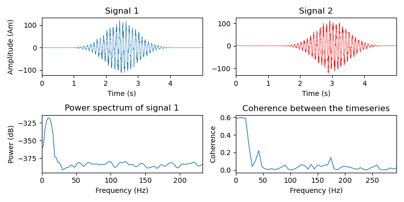
In the present example we shall devise a synthetic scenario in which two dipolar sources are active in the cortex. The source time courses are 10 Hz sinusoids, each modulated by a Gaussian. Simulated MEG recordings are then corrupted by empty room noise.

We shall use SESAME in the frequency domain [1] and see if we can find our two simulated sources.

References

[1]

G. Luria et al., Bayesian multi-dipole modelling in the frequency domain. J. Neurosci. Meth., 312 (2019) 27–36

# Author: Gianvittorio Luria <luria@dima.unige.it>
#
# License: BSD (3-clause)

import os.path as op
import numpy as np
from scipy.signal import welch, coherence
from matplotlib import pyplot as plt

import mne
from mne.datasets import sample

from sesameeg.mne import prepare_sesame


# We use the MEG and MRI setup from the MNE-Python
# sample dataset
data_path = sample.data_path(download=False)
subjects_dir = op.join(data_path, 'subjects')
subject = 'sample'

meg_path = op.join(data_path, 'MEG', 'sample')
raw_fname = op.join(meg_path, 'sample_audvis_raw.fif')
fwd_fname = op.join(meg_path, 'sample_audvis-meg-eeg-oct-6-fwd.fif')
erm_fname = op.join(meg_path, 'ernoise_raw.fif')
erm_cov_fname = op.join(meg_path, 'ernoise-cov.fif')

# Seed for the random number generator
rand = np.random.RandomState(42)

Load the info, the forward solution and the noise covariance The forward solution also defines the employed brain discretization.

info = mne.io.read_info(raw_fname)
fwd = mne.read_forward_solution(fwd_fname)
noise_cov = mne.read_cov(erm_cov_fname)

    Read a total of 3 projection items:
        PCA-v1 (1 x 102)  idle
        PCA-v2 (1 x 102)  idle
        PCA-v3 (1 x 102)  idle
Reading forward solution from /home/pasca/mne_data/MNE-sample-data/MEG/sample/sample_audvis-meg-eeg-oct-6-fwd.fif...
    Reading a source space...
    Computing patch statistics...
    Patch information added...
    Distance information added...
    [done]
    Reading a source space...
    Computing patch statistics...
    Patch information added...
    Distance information added...
    [done]
    2 source spaces read
    Desired named matrix (kind = 3523) not available
    Read MEG forward solution (7498 sources, 306 channels, free orientations)
    Desired named matrix (kind = 3523) not available
    Read EEG forward solution (7498 sources, 60 channels, free orientations)
    Forward solutions combined: MEG, EEG
    Source spaces transformed to the forward solution coordinate frame
    306 x 306 full covariance (kind = 1) found.
    Read a total of 3 projection items:
        PCA-v1 (1 x 102) active
        PCA-v2 (1 x 102) active
        PCA-v3 (1 x 102) active

In this example, to save computation time, we shall only simulate gradiometer data. You can try simulating other types of sensors as well.

picks = mne.pick_types(info, meg='grad', stim=True, exclude='bads')
mne.pick_info(info, picks, copy=False)
fwd = mne.pick_channels_forward(fwd, include=info['ch_names'])
noise_cov = mne.pick_channels_cov(noise_cov, include=info['ch_names'])

203 out of 366 channels remain after picking

Data simulation

The following function generates a timeseries that contains an oscillator, modulated by a Gaussian. The frequency of the oscillator fluctuates a little over time, but stays close to 10 Hz.

def gen_signal(times, base_freq, rand=None, t_rand=1e-3, std_rand=0.1, g_sigma=None, g_mu_shift=None):
    """Generate an oscillating signal with a Gaussian envelope.

    Parameters
    ----------
    times : array
        Times
    base_freq : float
        Base frequency of the oscillators in Hertz
    t_rand : float
        Variation in the instantaneous frequency of the signal
    std_rand : float
        Std-dev of the random fluctuations added to the signal
    g_sigma : float
        Standard deviation of the enveloping Gaussian
    g_mu_shift: float
        Shift (in seconds) of the mean of the enveloping Gaussian with respect to the
        middle of the time window

    Returns
    -------
    signal : ndarray
        The generated signal.
    """

    n_times = len(times)

    mu_0 = np.floor(times.shape[0] / 2)
    mu_shift = int(g_mu_shift * sfreq)
    mu = int(mu_0 + mu_shift) / sfreq
    gauss = np.exp(-np.power(times - mu, 2.) / (2 * np.power(g_sigma, 2.)))

    if rand is not None:
        # Generate an oscillator with varying frequency and phase lag.
        signal = np.sin(2.0 * np.pi * (base_freq * np.arange(n_times) / sfreq +
                                       np.cumsum(t_rand * rand.randn(n_times))))

        # Add some random fluctuations to the signal.
        signal += std_rand * rand.randn(n_times)
    else:
        signal = np.sin(2.0 * np.pi * (base_freq * np.arange(n_times) / sfreq +
                                       np.cumsum(t_rand * np.random.randn(n_times))))
        signal += std_rand * np.random.randn(n_times)

    # Scale the signal to be in the right order of magnitude (~100 nAm)
    # for MEG data.
    signal *= 100e-9 * gauss

    return signal

We now simulate two timeseries and plot some basic information about them.

sfreq = info['sfreq']
n_sample = int(round(5. * sfreq))
times = np.arange(n_sample) / sfreq
signal1 = gen_signal(times, 10., g_sigma=.5, g_mu_shift=0)
signal2 = gen_signal(times, 10., g_sigma=.5, g_mu_shift=.5)
q = np.vstack((signal1, signal2))

fig, axes = plt.subplots(2, 2, figsize=(8, 4))

# Plot the timeseries
ax = axes[0][0]
ax.plot(times, 1e9 * signal1, lw=0.5)
ax.set(xlabel='Time (s)', xlim=times[[0, -1]], ylabel='Amplitude (Am)',
       title='Signal 1')
ax = axes[0][1]
ax.plot(times, 1e9 * signal2, lw=0.5, color = 'r')
ax.set(xlabel='Time (s)', xlim=times[[0, -1]], title='Signal 2')

# Power spectrum of the first timeseries
f, p = welch(signal1, fs=sfreq, nperseg=128, nfft=256)
ax = axes[1][0]
# Only plot the first 100 frequencies
ax.plot(f[:100], 20 * np.log10(p[:100]), lw=1.)
ax.set(xlabel='Frequency (Hz)', xlim=f[[0, 99]],
       ylabel='Power (dB)', title='Power spectrum of signal 1')

# Compute the coherence between the two timeseries
f, coh = coherence(signal1, signal2, fs=sfreq, nperseg=100, noverlap=64)
ax = axes[1][1]
ax.plot(f[:50], coh[:50], lw=1.)
ax.set(xlabel='Frequency (Hz)', xlim=f[[0, 49]], ylabel='Coherence',
       title='Coherence between the timeseries')
fig.tight_layout()

Now we put the signals at two locations on the cortex. To do so, we construct a mne.SourceEstimate object to store them in.

# The locations on the cortex where the signal will originate from are
# indicated as source space grid points indices.
vertices = [[146374], [33830]]
vertno = np.hstack([fwd['src'][0]['vertno'], fwd['src'][1]['vertno']])
true_locs = list()
for v in vertices:
    true_locs.append(np.where(vertno == v[0])[0][0])

# Construct SourceEstimates that describe the signals at the cortical level.
stc_signal = mne.SourceEstimate(q, vertices, tmin=0, tstep=1. / sfreq, subject='sample')

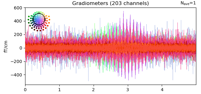
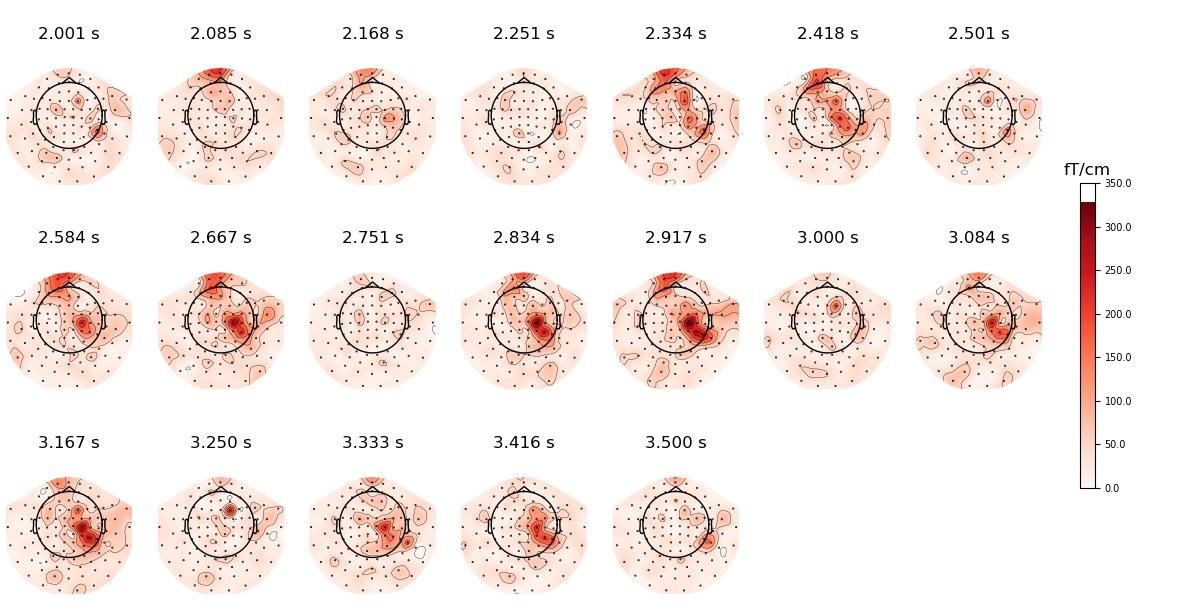
Now we run the signal through the forward model to obtain simulated sensor data. We then corrupt the resulting simulated gradiometer recordings by empty room noise.

evoked = mne.apply_forward(fwd, stc_signal, info)
mne.simulation.add_noise(evoked, noise_cov, random_state=rand)

    Average patch normals will be employed in the rotation to the local surface coordinates....
    Converting to surface-based source orientations...
    [done]
/home/pasca/Tools/python/packages/sesameeg/examples/plot_06_compute_sesame_meg_simulated_frequency_mne.py:180: RuntimeWarning: The maximum current magnitude is 121.2 nAm, which is very large. Are you trying to apply the forward model to noise-normalized (dSPM, sLORETA, or eLORETA) values? The result will only be correct if currents (in units of Am) are used.
  evoked = mne.apply_forward(fwd, stc_signal, info)
Projecting source estimate to sensor space...
[done]
Adding noise to 203/203 channels (203 channels in cov)

Condition
Data kind	average
Timepoints	3003 samples
Channels	203 channels
Number of averaged epochs	1
Time range (secs)	0.0 – 4.998210249179003
Baseline (secs)	off

Visualize the data

evoked.plot()
_t = evoked.times[(2.0 < evoked.times) & (evoked.times < 3.5)]
evoked.plot_topomap(times=_t[::50], nrows=3)
plt.show()

• 
• 

Define the parameters and apply SESAME. We convert the data to the frequency domain by setting fourier=True.

n_parts = 100
noise_std = None
dip_mom_std = None
freq_min = 9.5
freq_max = 10.5

_sesame = prepare_sesame(fwd, evoked, n_parts=n_parts, noise_std=noise_std,
                         top_min=freq_min, top_max=freq_max, dip_mom_std=dip_mom_std,
                         hyper_q=True, fourier=True, subject=subject, subjects_dir=subjects_dir)

_sesame.apply_sesame()
print('    Estimated source locations: {0}'.format(_sesame.est_locs[-1]))
print('    True source locations: {0}'.format(true_locs))

# Compute goodness of fit
gof = _sesame.goodness_of_fit()
print('    Goodness of fit with the recorded data: {0}%'.format(round(gof, 4) * 100))

# Compute source dispersion
sd = _sesame.source_dispersion()
print('    Source Dispersion: {0} mm'.format(round(sd, 2)))

Computing inverse operator with 203 channels.
    203 out of 203 channels remain after picking
Forward model with free source orientation.
Computing neighbours matrix [done]
Computing neighbours probabilities...[done]
Data have been converted to the frequency domain.
Analyzing data from 9.6002 Hz to 10.4003 Hz
Estimating dipole moment std...[done]
 Estimated dipole moment std: 2.1725e-05
Sampling hyperprior for dipole moment std.
Estimating noise std...[done]
 Estimated noise std: 2.6864e-09
Computing inverse solution. This will take a while...
/home/pasca/Tools/python/packages/sesameeg/sesameeg/particles.py:174: RuntimeWarning: invalid value encountered in log
  self.loglikelihood_unit = - (n_ist * noise_std**2) * np.log(det_sigma)
/home/pasca/mambaforge/envs/mne_15/lib/python3.11/site-packages/numpy/linalg/linalg.py:2139: RuntimeWarning: overflow encountered in det
  r = _umath_linalg.det(a, signature=signature)
Estimated dipole strength variance: 9.466076567752923e-06
    Estimated number of sources: 2
    Estimated source locations:
        * source 1: [0.02482721 0.00881952 0.12250079]
        * source 2: [-0.0283287   0.09554572  0.05893362]
[done in 88 iterations]
    Estimated source locations: [4367 3554]
    True source locations: [3554, 4367]
    Goodness of fit with the recorded data: 92.44%
    Source Dispersion: 1.37 mm

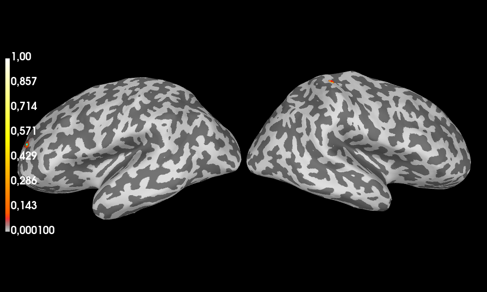
Visualize the posterior map of the dipoles’ location and the estimated sources on the inflated brain. If window closes unexpectedly, set force_open=True

_sesame.plot_sources(true_sources=true_locs, force_open=False, plot_kwargs={'distance': 650})

Surface stc computed.
[3554, 4367]