Explore SESAME alternative inverse solutions on evoked data

In this example we shall show that SESAME is able to provide alternative solutions with non-negligible probabilities and how the user can easily explore all of them.

To do so, we shall once again apply SESAME on an evoked dataset, corresponding to the response to an auditory stimulus. Data are taken from the MNE-Python sample dataset.

# Author: Gianvittorio Luria <luria@dima.unige.it>
#
# License: BSD (3-clause)

# sphinx_gallery_thumbnail_number = 2

from os import path as op
import numpy as np
import matplotlib.pyplot as plt

from mne.datasets import sample
from mne import read_forward_solution, pick_types_forward, read_evokeds

from sesameeg.mne import prepare_sesame

data_path = sample.data_path()
subject = 'sample'
subjects_dir = op.join(data_path, 'subjects')
fname_fwd = op.join(data_path, 'MEG', subject,
                    'sample_audvis-meg-eeg-oct-6-fwd.fif')
fname_evoked = op.join(data_path, 'MEG', subject, 'sample_audvis-ave.fif')

Load the forward solution and the evoked data . The forward solution also defines the employed brain discretization.

meg_sensor_type = True  # All MEG sensors will be included
eeg_sensor_type = False

# Forward solution
fwd = read_forward_solution(fname_fwd, exclude='bads')
fwd = pick_types_forward(fwd, meg=meg_sensor_type,
                         eeg=eeg_sensor_type, ref_meg=False)

# Evoked Data
condition = 'Left Auditory'
evoked = read_evokeds(fname_evoked, condition=condition, baseline=(None, 0))
evoked = evoked.pick('meg', exclude='bads')

Reading forward solution from /home/pasca/mne_data/MNE-sample-data/MEG/sample/sample_audvis-meg-eeg-oct-6-fwd.fif...
    Reading a source space...
    Computing patch statistics...
    Patch information added...
    Distance information added...
    [done]
    Reading a source space...
    Computing patch statistics...
    Patch information added...
    Distance information added...
    [done]
    2 source spaces read
    Desired named matrix (kind = 3523) not available
    Read MEG forward solution (7498 sources, 306 channels, free orientations)
    Desired named matrix (kind = 3523) not available
    Read EEG forward solution (7498 sources, 60 channels, free orientations)
    Forward solutions combined: MEG, EEG
    Source spaces transformed to the forward solution coordinate frame
    364 out of 366 channels remain after picking
    305 out of 364 channels remain after picking
Reading /home/pasca/mne_data/MNE-sample-data/MEG/sample/sample_audvis-ave.fif ...
    Read a total of 4 projection items:
        PCA-v1 (1 x 102) active
        PCA-v2 (1 x 102) active
        PCA-v3 (1 x 102) active
        Average EEG reference (1 x 60) active
    Found the data of interest:
        t =    -199.80 ...     499.49 ms (Left Auditory)
        0 CTF compensation matrices available
        nave = 55 - aspect type = 100
Projections have already been applied. Setting proj attribute to True.
Applying baseline correction (mode: mean)
Removing projector <Projection | Average EEG reference, active : True, n_channels : 60>

Define the parameters.

time_min, time_max = 0.045, 0.135  # Select N100m
sample_min, sample_max = evoked.time_as_index([time_min, time_max],
                                              use_rounding=True)

# Fix the random seed
np.random.seed(3)

# Manually set the noise standard deviation value. We are intentionally
# overestimating the parameter with respect to SESAME’s default.
noise_std = 0.64 * np.max(abs(evoked.data))

# If None, dip_mom_std will be estimated by SESAME.
dip_mom_std = None

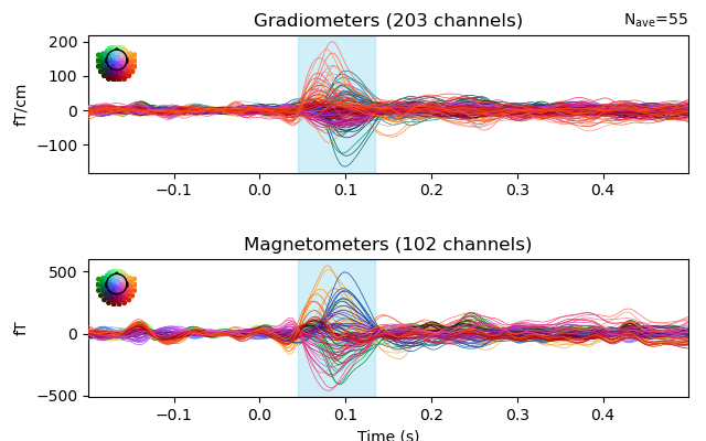
Visualize the selected data.

fig = evoked.plot(show=False)
for ax in fig.get_axes()[:2]:
    ax.axvspan(time_min, time_max, alpha=0.3, color="#66CCEE")
plt.show()

Apply SESAME.

_sesame = prepare_sesame(fwd, evoked, noise_std=noise_std,
                         top_min=time_min, top_max=time_max,
                         dip_mom_std=dip_mom_std, hyper_q=True,
                         subject=subject, subjects_dir=subjects_dir)
_sesame.apply_sesame()


# Compute goodness of fit
gof = _sesame.goodness_of_fit()
print('    Goodness of fit with the recorded data: {0}%'.format(round(gof, 4) * 100))

# Compute source dispersion
sd = _sesame.source_dispersion()
print('    Source Dispersion: {0} mm'.format(round(sd, 2)))

Computing inverse operator with 305 channels.
    305 out of 305 channels remain after picking
Forward model with free source orientation.
Computing neighbours matrix [done]
Computing neighbours probabilities...[done]
Analyzing data from 0.045 s to 0.1349 s
Estimating dipole moment std...[done]
 Estimated dipole moment std: 3.2335e-08
Sampling hyperprior for dipole moment std.
User defined noise std: 1.2795e-11
Computing inverse solution. This will take a while...
/home/pasca/Tools/python/packages/sesameeg/sesameeg/particles.py:174: RuntimeWarning: invalid value encountered in log
  self.loglikelihood_unit = - (n_ist * noise_std**2) * np.log(det_sigma)
Estimated dipole strength variance: 1.5377524946735598e-08
    Estimated number of sources: 1
    Estimated source locations:
        * source 1: [0.04930186 0.0095755  0.06843461]
[done in 45 iterations]
    Goodness of fit with the recorded data: 21.41%
    Source Dispersion: 3.68 mm

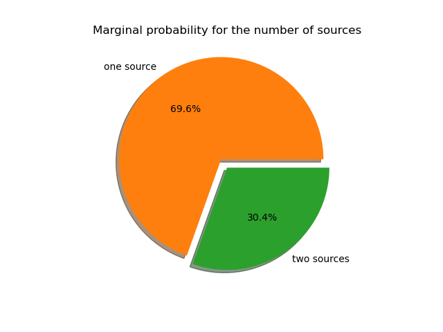
Visualize the marginal probability of the number of sources

_sesame.plot_source_number(kind='pie')

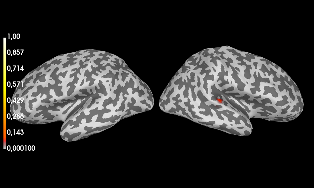
Visualize the posterior map of the dipoles’ location and the estimated sources on the inflated brain.

_sesame.plot_sources(plot_kwargs={'distance': 650})

Surface stc computed.

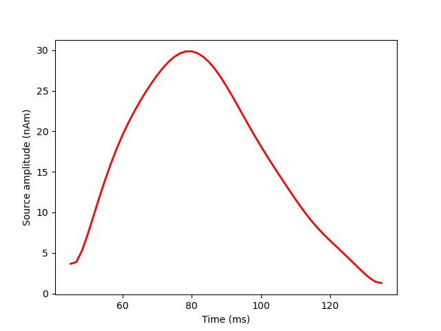
Visualize the amplitude of the estimated sources as function of time.

_sesame.plot_source_amplitudes()

Explore the alternative scenario

_sesame.plot_sources(n_sources=2, plot_kwargs={'distance': 650})
_sesame.plot_source_amplitudes(n_sources=2)

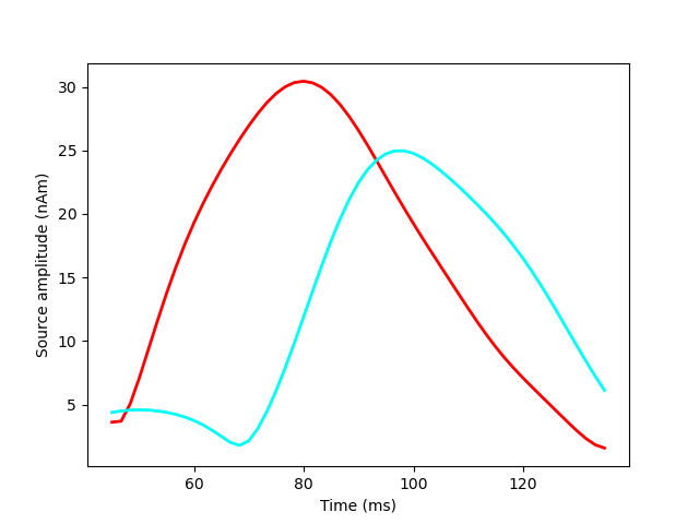
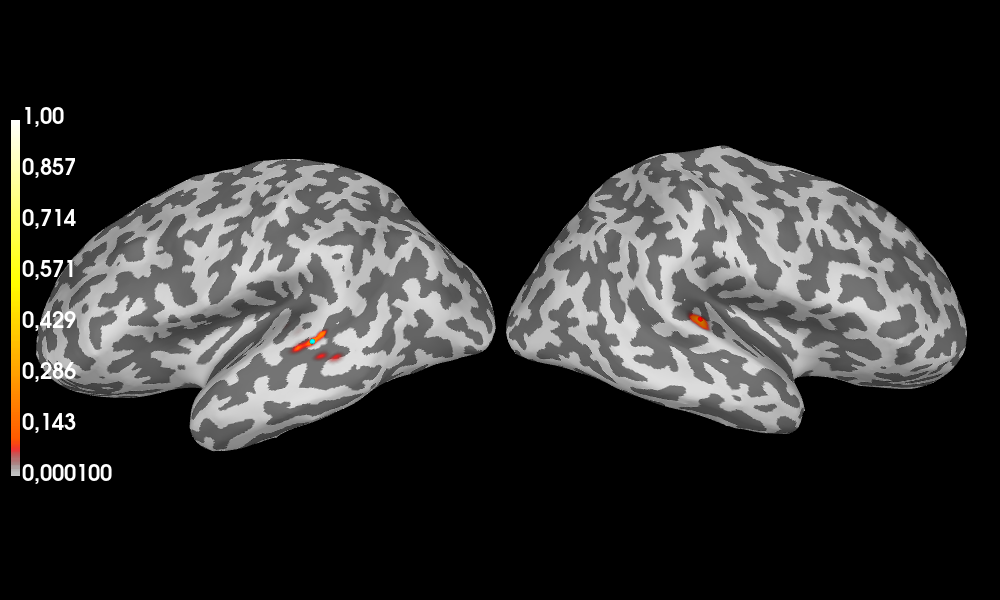
Computing point estimates for user defined source configuration.
    Selected number of sources: 2
    Estimated source locations:
        * source 1: [0.04930186 0.0095755  0.06843461]
        * source 2: [-0.05630193  0.00230887  0.05666819]
Surface stc computed.
Computing point estimates for user defined source configuration.