Compute SESAME inverse solution on high-density EEG data

In the present example we shall show how to perform a source modeling analysis using SESAME as a standalone software.

The data belongs to a recently published EEG dataset of high-density (256 channels) scalp recordings combined with a ground truth single dipolar source systematically provided through a brief current injection between two adjacent intracranial electrodes whose position is known with millimetric precision [1] [2] .

References

[1]

Mikulan et al., Simultaneous human intracerebral stimulation and HD-EEG, ground-truth for source localization methods. Sci Data, 7 (2020)

[2]

Pascarella et al., An in–vivo validation of ESI methods with focal sources. NeuroImage, 277 (2023)

# Author: Gianvittorio Luria <luria@dima.unige.it>
#
# License: BSD (3-clause)

# sphinx_gallery_thumbnail_number = 2

import numpy as np
import scipy.io as sio
import scipy.spatial.distance as ssd
import matplotlib.pyplot as plt
from sesameeg import Sesame

Import the MATLAB data structure and extract the single quantities.

data_mat = sio.loadmat('data/sub-01_run-07_data.mat')

source_space = data_mat['src_coo']
good_chs = data_mat['good_chs'][0] - 1
lead_field = data_mat['LF'][good_chs]
data = data_mat['evoked']
data_times = data_mat['times'][0]
true_coords = np.array([0.034775, -0.00336, 0.039735])
true_sources = [np.argmin(ssd.cdist(source_space, true_coords.reshape(1, -1))[:, 0])]

Define the parameters.

sample_min, sample_max = 12, 24
subsample = None

# To accelerate the run time of this example, we use a small number of
# particles. We recall that the parameter ``n_parts`` represents, roughly speaking,
# the number of candidate solutions that are tested in the Monte Carlo procedure;
# larger values yield in principle more accurate reconstructions but also entail a
# higher computational cost. Setting the value to about a hundred seems to represent
# a good trade–off.
n_parts = 10
# If None, noise_std and dip_mom_std will be estimated by SESAME.
noise_std = None
dip_mom_std = None

Visualize the selected data.

plt.figure(figsize=(25,8))
plt.plot(data_times, data.T, label='EEG data')
plt.axvspan(data_times[sample_min], data_times[sample_max], alpha=0.2, label='Analyzed data')
plt.xlabel('Time')
plt.title(f'EEG Data ({data.shape[0]} channels)')
plt.show()

Apply SESAME.

_sesame = Sesame(source_space, lead_field, data, n_parts=n_parts, noise_std=noise_std,
                 s_max=sample_max, s_min=sample_min, dip_mom_std=dip_mom_std,
                 hyper_q=True, subsample=subsample, data_times=data_times)

_sesame.apply_sesame()

# Compute goodness of fit
gof = _sesame.goodness_of_fit()
print('    Goodness of fit with the recorded data: {0}%'.format(round(gof, 4) * 100))

# Compute source dispersion
sd = _sesame.source_dispersion()
print('    Source Dispersion: {0} mm'.format(round(sd, 2)))

# Compute distance to true source
distance = ssd.cdist(source_space[_sesame.est_locs[-1][0]].reshape(1,-1), true_coords.reshape(1,-1))[0][0]
print('    Distance to true source: {0} mm'.format(round(distance*1000, 2)))

Computing neighbours matrix [done]
Computing neighbours probabilities...[done]
Estimating dipole moment std...[done]
 Estimated dipole moment std: 2.1657e-06
Sampling hyperprior for dipole moment std.
Estimating noise std...[done]
 Estimated noise std: 2.8010e-04
Computing inverse solution. This will take a while...
/home/pasca/Tools/python/packages/sesameeg/sesameeg/particles.py:174: RuntimeWarning: invalid value encountered in log
  self.loglikelihood_unit = - (n_ist * noise_std**2) * np.log(det_sigma)
Estimated dipole strength variance: 2.20030636474554e-06
    Estimated number of sources: 1
    Estimated source locations:
        * source 1: [ 0.03371428 -0.00413685  0.03588749]
[done in 64 iterations]
    Goodness of fit with the recorded data: 78.89%
    Source Dispersion: 3.18 mm
    Distance to true source: 4.07 mm

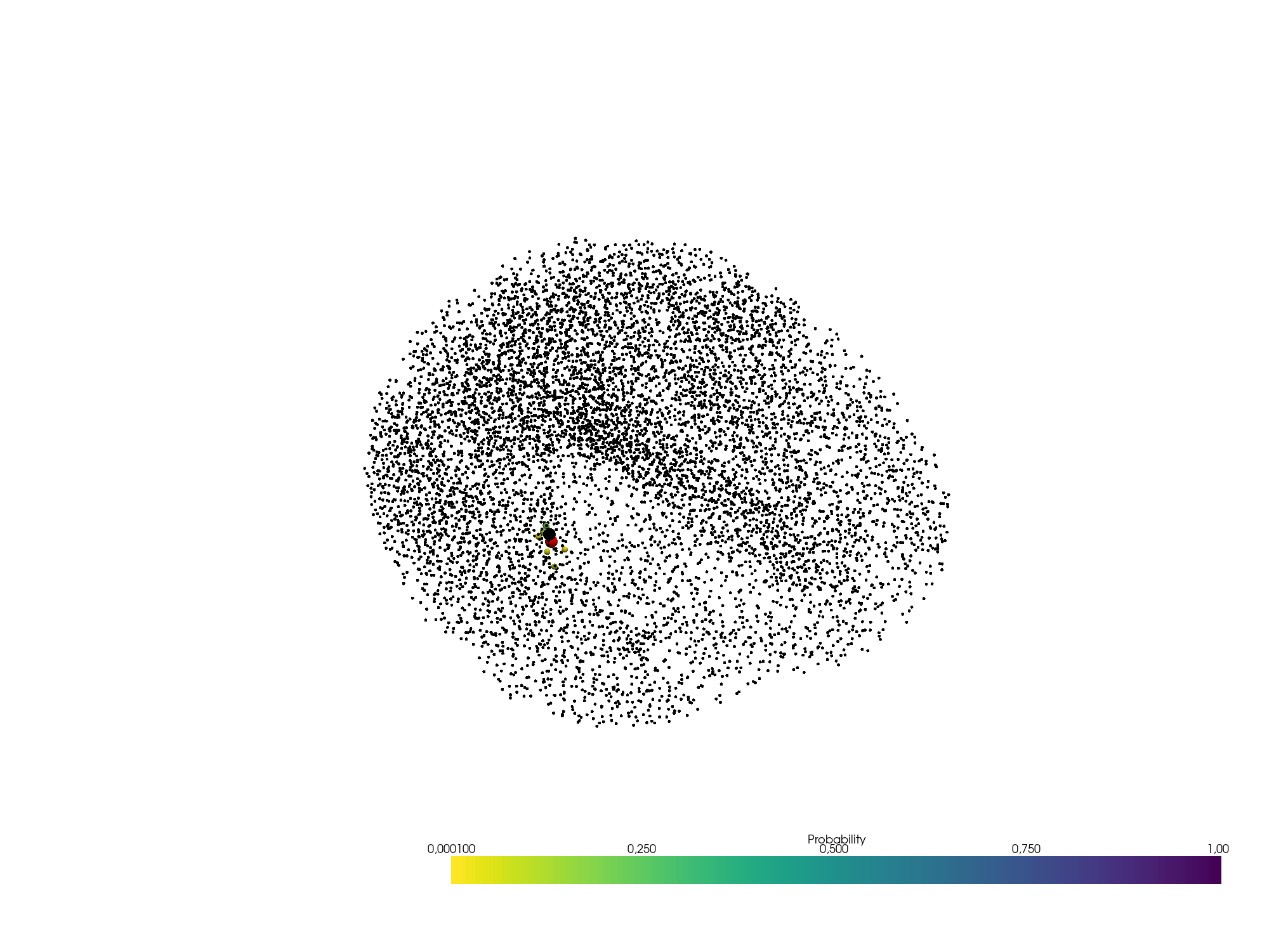
Visualize the posterior map of the dipoles’ location and the estimated sources on the inflated brain.

_sesame.plot_sources(true_sources=true_sources)

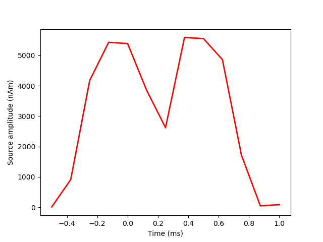
Visualize the amplitude of the estimated sources as function of time.

_sesame.plot_source_amplitudes()

Save results.

# You can save SESAME result in an HDF5 file with:
# _sesame.save_h5(save_fname, sbj=subject, data_path=fname_evoked, fwd_path=fname_fwd)

# You can save SESAME result in a Pickle file with:
# _sesame.save_pkl(save_fname, sbj=subject, data_path=fname_evoked, fwd_path=fname_fwd)